VLOOKUP Formula In Excel with Example PDF
Microsoft Office (MS) Excel has large number of functions and utilities which an average user forget to use them. User can also make their own formulas. If you have one big database in which you want to find the cost of an item quickly, then user can use VLOOKUP function quickly. If you search in a database to obtain only one kind of data, then user should learn the usage of VLOOKUP.
What is VLOOKUP in Excel With Example?
VLOOKUP is one of the best function in MS Excel. We use this formula to see usually a special value in a big database where manual search become troublesome.
VLOOKUP function is also support approximate, exact match and wildcard (*?) match.
Meaning of Excel VLOOKUP
V mean is “Vertical”. We can use this to see the value vertically. So its use can be done to see the value inside of any cell of column.
Syntax of VLOOKUP Function
The syntax of VLOOKUP function is made by four type of information.
= VLOOKUP (value, table, col_index, [range_lookup])
Below arguments exists in VLOOKUP fomula.
value : value of first column available in table to which we want to search. (Lookup_value). Note : Keep remember that lookup value should always in first column of range so that it can work better.
table : table from which we want to retrieve this value (i.e. a range in which this value exists.) (Table_array)
col_index : the column of a table of range from which value need to obtain. (Col_index_num). In this, there are two options of range_lookup – [True (1) = Approximate Match, False(0) = Exact Match]. If you will not enter any col_index_num, it will take True (1) by default.
How Excel VLOOKUP Function works?
Before using the VLOOKUP, we should first understand the way of function of VLOOKUP.
VLOOKUP is designed to retrieve the organised data from vertical rows of table where each row represents a new record.
If your data is organised horizontally, then use the HLOOKUP function.
How to use Excel VLOOKUP?
Before understanding the way of usage of VLOOKUP function, we must understand what is the aim of this. We will try to understand by one sample problem.
Suppose, we have one table which is shown below.

Now remember the below three points to use the VLOOKUP function.
(i) VLOOKUP Only Looks Right
VLOOKUP see only toward the right of the VLOOKUP value column. VLOOKUP has needed such table in which lookup value is in the leftmost column.
Whatever data you want to retrieve like salary that should be in the any right columns of Id.

(ii) VLOOKUP Retrieves Data Based On Column Number
When you use the VLOOKUP, understand that numbered the column from left in the selected range. Like we cannot retrieve the name from the above table. Because we are getting the Salary based on the Id but Name is not right side of Id column.

In case of 107, =VLOOKUP(G3,C3:E8,2,0) [Department] & =VLOOKUP(G3,C3:E8,3,0) [Salary]
In case of 101, =VLOOKUP(G4,C4:E9,2,0) [Department] & =VLOOKUP(G4,C4:E9,3,0) [Salary]
iii). VLOOKUP has two matching modes, exact and approximate
VLOOKUP has two modes : matching : exact and approximate which is controlled by fourth argument called “range_lookup”.
Enter “False (0) for exact match in the range_lookup” or “True (1) for approximate match in range_lookup”. By default value of range_lookup, it will be approximate match i.e. if you have not provided the fourth argument, it will find the approximate value.
=VLOOKUP(Lookup_value, Table_array,Col_index_num) //By default, approximate match
=VLOOKUP(Lookup_value, Table_array,Col_index_num, TRUE) //approximate match
=VLOOKUP(Lookup_value, Table_array,Col_index_num, FALSE) //exact match
VLOOKUP is an inbuilt formula, you can find this Insert Function sign as given below in screenshot.

After that you will find the Insert Function dialog and you need to search for VLOOKUP. So type the VLOOKUP in (Search for a function) box and click on Go.

Now click on OK button. Below are the arguments with explanation.
Lookup_value = is the value to be found in the first column of the table, and can be a value, a reference, or a text string.
Table_array = is a table of text, numbers, or logical values, in which data is retrieved. Table_array can be a reference to a range or a range name.
Col_index_num = is the column number in table_array from which the matching value should be returned. The first column of values in the table is column 1.
Range_lookup = is a logical value: to find the closest match in the first column. (i.e. sorted in ascending order) = TRUE or omitted; find an exact match = FALSE.
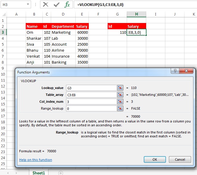
After pressing OK. You will find the salary of Id 110 as 70000. If you want to find the salary of any employee further, just change the 110 with the desired Id. You will find the salary of that desired number.
VLOOKUP Between WorkSheets & Workbooks
Find the vlookup value between the workbooks and worksheets. Ensure that both the excel files are open on the same computer.
Consider, i want to get salary from the table available in sheet 1 on the sheet 2 in column B2. Then Formula will be like below.
= VLOOKUP (B2, “Sheet1”!$C$3:$E$8,3,0)
Consider if i want to obtain the salary from another excel (workbook) named “vlookup-between_multiple_files_B.xlx”, then formula will be like given below.
= VLOOKUP (B2, “[vlookup-between_multiple_files_B.xlx]Sheet1”!$C$3:$E$8,3,0)
VLOOKUP Formula In Excel with Example PDF Download
Candidates can download the above full details in excel by clicking on below link.
Hope you understand well. Good Luck
Very interesting information!Perfect just what I was looking for!